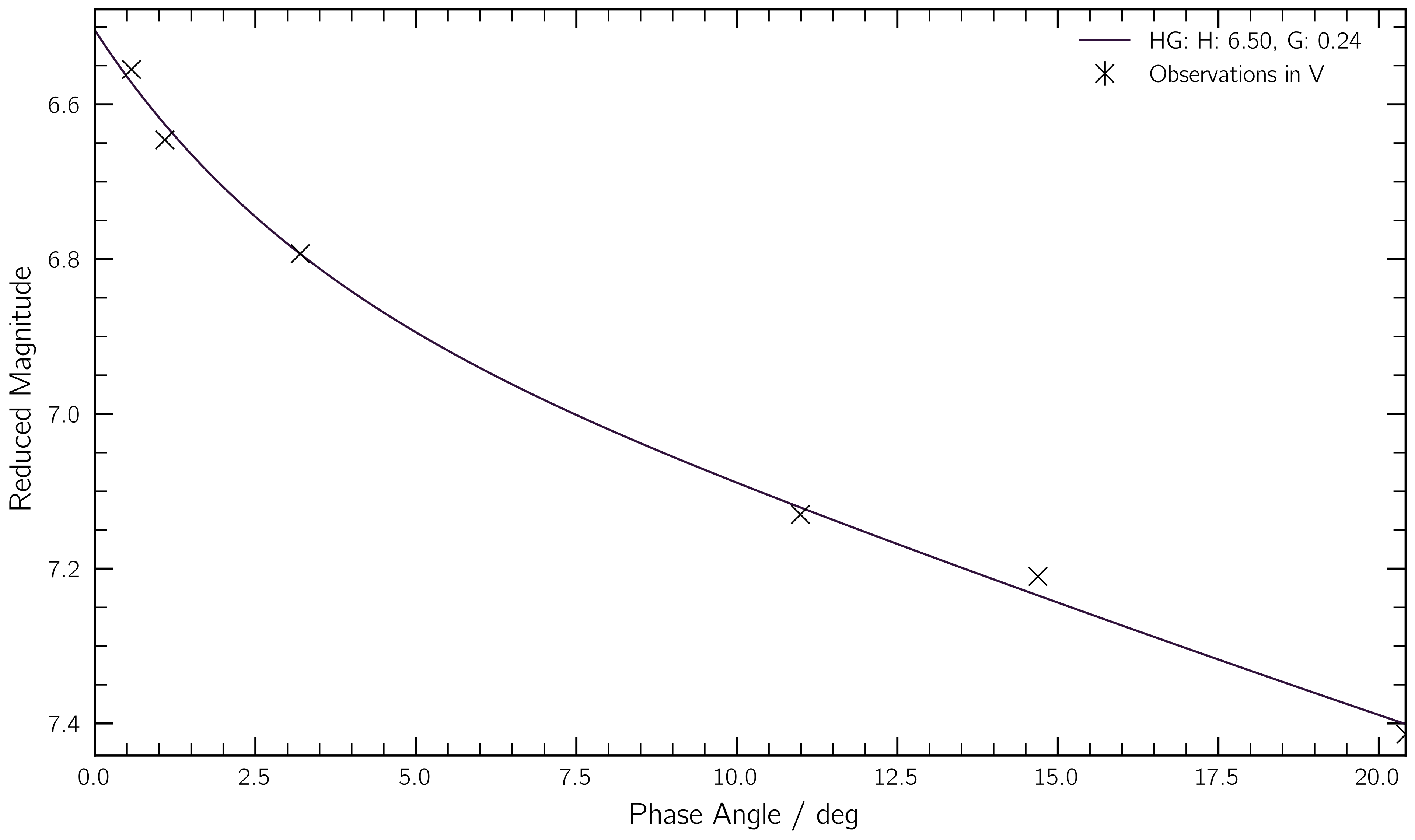
Photometric Models¶

HG¶

From Bowell+ 1989. phunk uses the model implementation from sbpy.

import phunk

# Observations of (20) Massalia from Gehrels 1956
phase = [0.57, 1.09, 3.20, 10.99, 14.69, 20.42]
mag = [6.555, 6.646, 6.793, 7.130, 7.210, 7.414]

pc = phunk.PhaseCurve(phase=phase, mag=mag)
pc.fit(['HG'])

pc.plot()

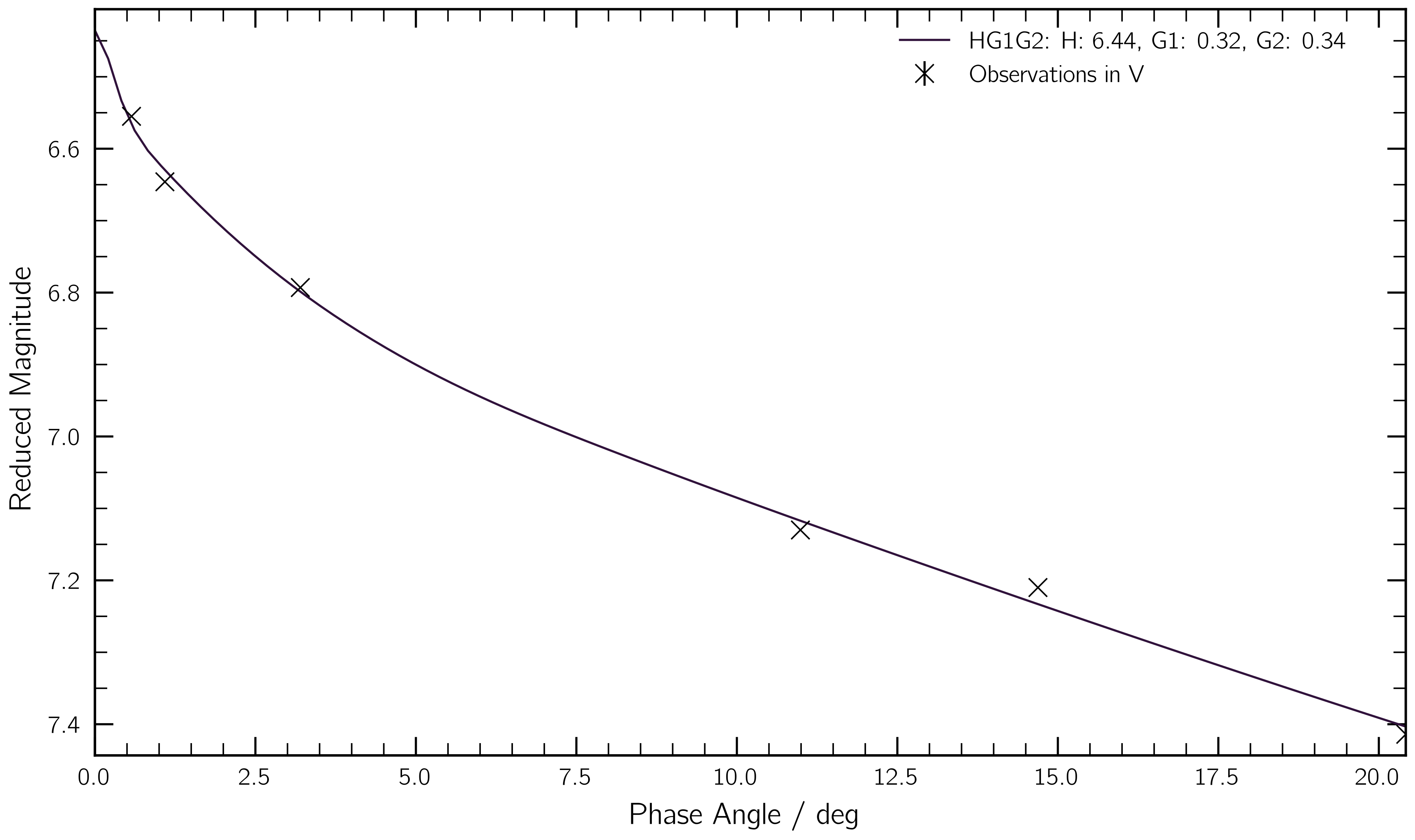
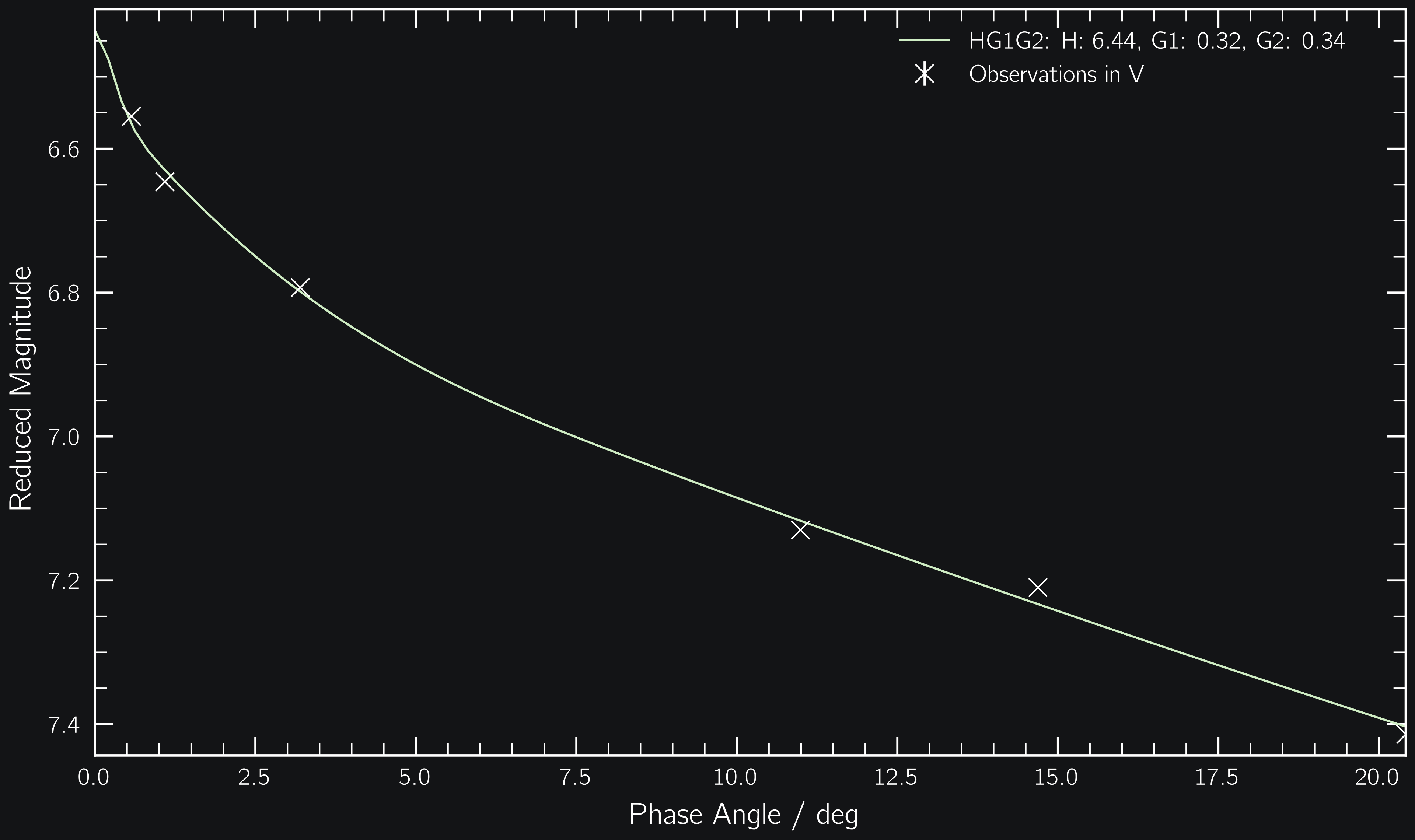
HG1G2¶

From Muinonen+ 2010. phunk uses the model implementation from sbpy.

import phunk

# Observations of (20) Massalia from Gehrels 1956
phase = [0.57, 1.09, 3.20, 10.99, 14.69, 20.42]
mag = [6.555, 6.646, 6.793, 7.130, 7.210, 7.414]

pc = phunk.PhaseCurve(phase=phase, mag=mag)
pc.fit(['HG1G2'])

pc.plot()

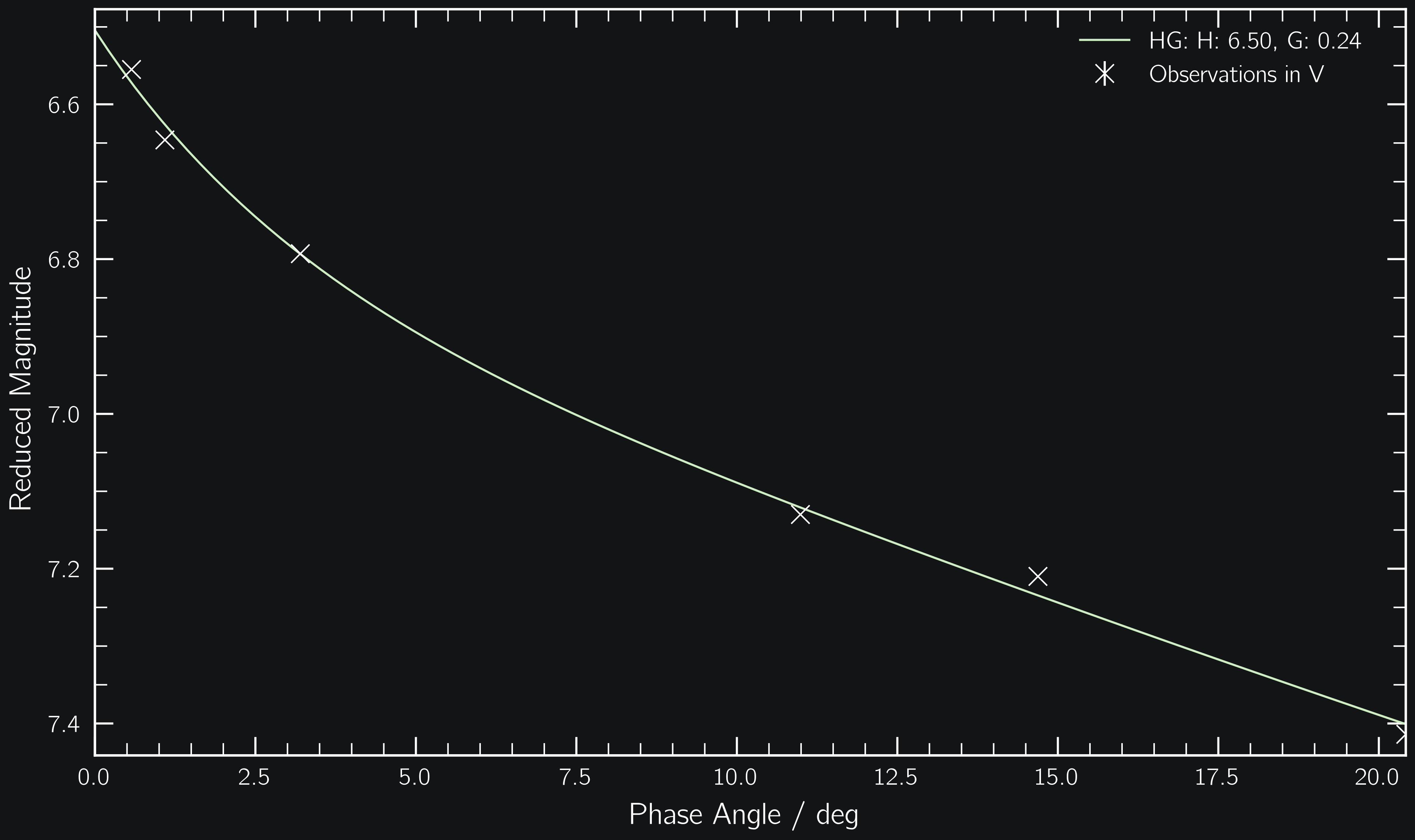
HG12¶

From Muinonen+ 2010. phunk uses the model implementation from sbpy.

import phunk

# Observations of (20) Massalia from Gehrels 1956
phase = [0.57, 1.09, 3.20, 10.99, 14.69, 20.42]
mag = [6.555, 6.646, 6.793, 7.130, 7.210, 7.414]

pc = phunk.PhaseCurve(phase=phase, mag=mag)
pc.fit(['HG'])

pc.plot()

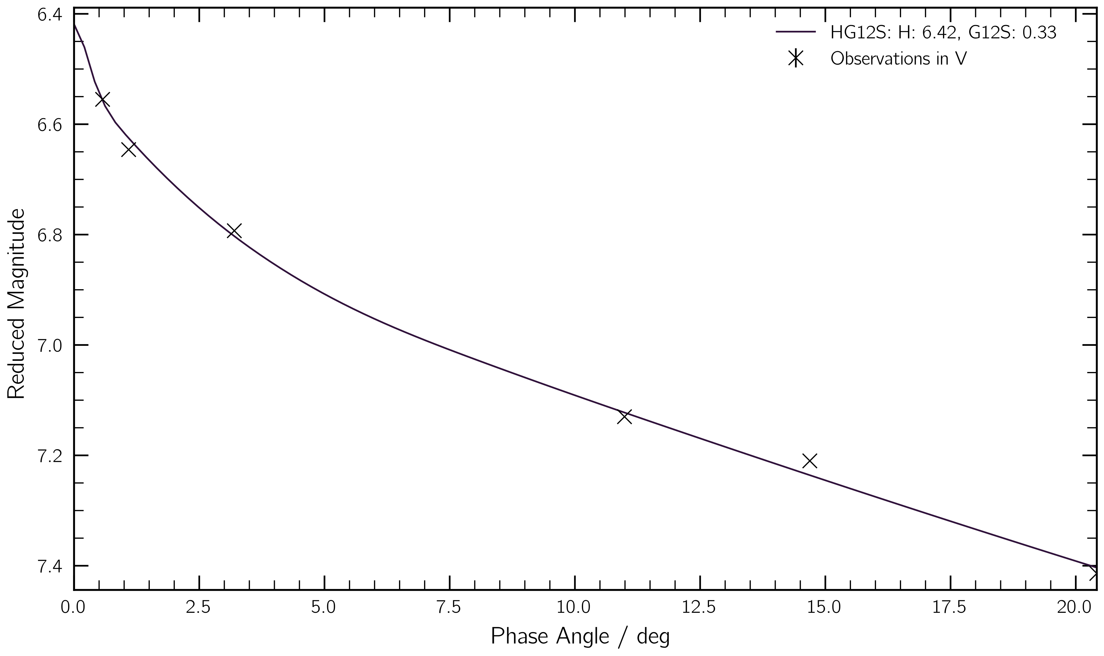
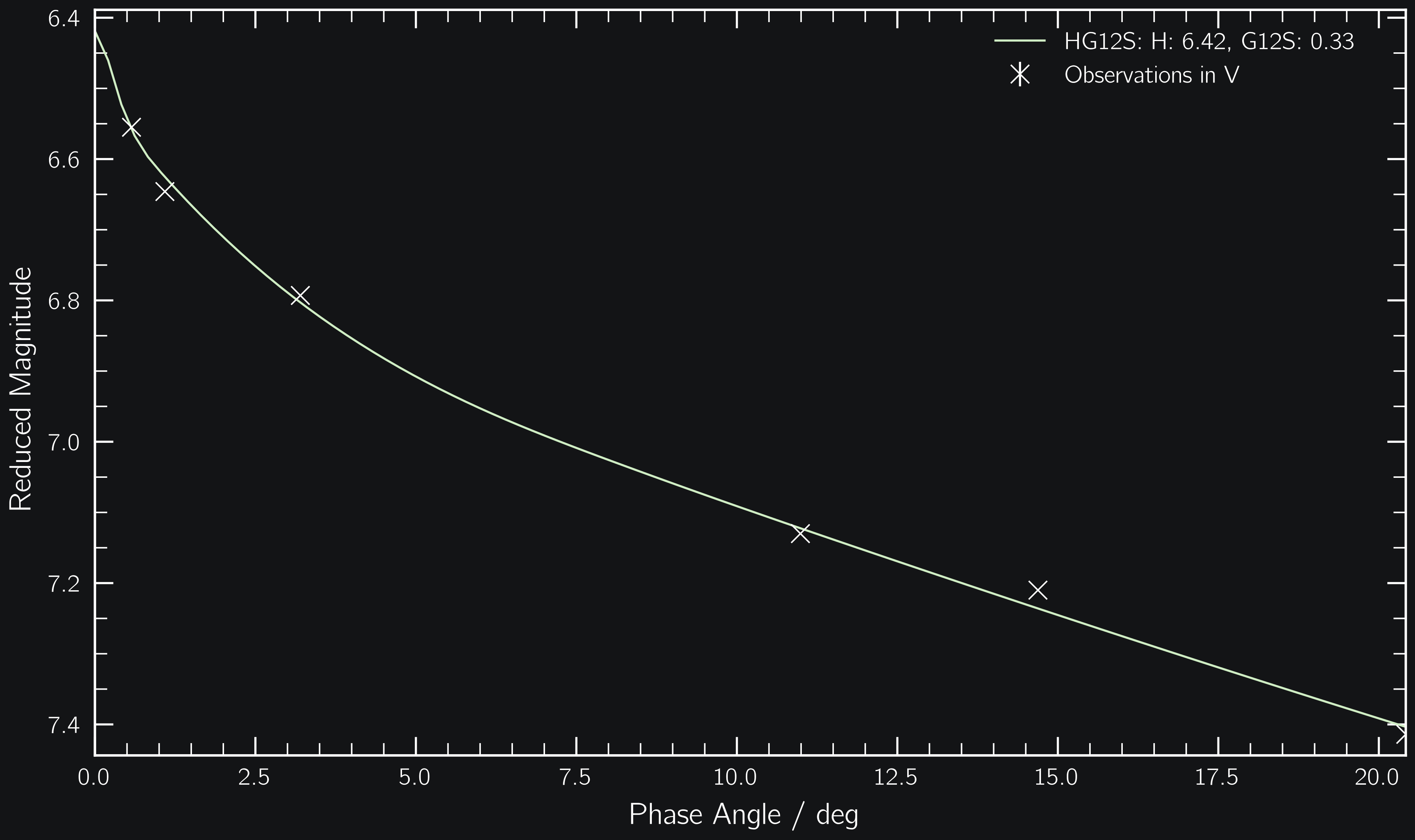
HG12S¶

From Penttilä+ 2016. In the paper, it is called the HG12* model. phunk uses the model implementation from sbpy.

import phunk

# Observations of (20) Massalia from Gehrels 1956
phase = [0.57, 1.09, 3.20, 10.99, 14.69, 20.42]
mag = [6.555, 6.646, 6.793, 7.130, 7.210, 7.414]

pc = phunk.PhaseCurve(phase=phase, mag=mag)
pc.fit(['HG12S'])

pc.plot()

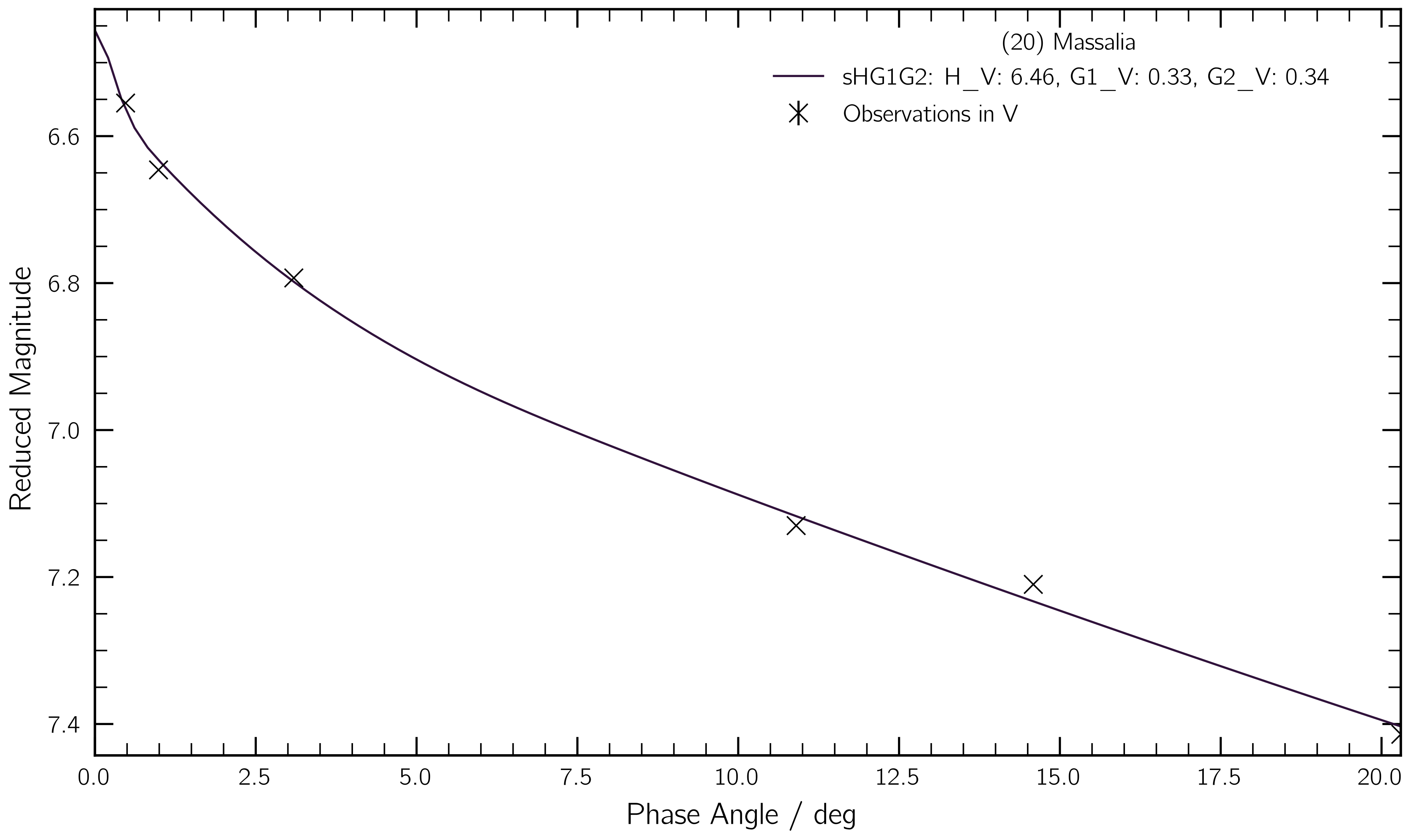
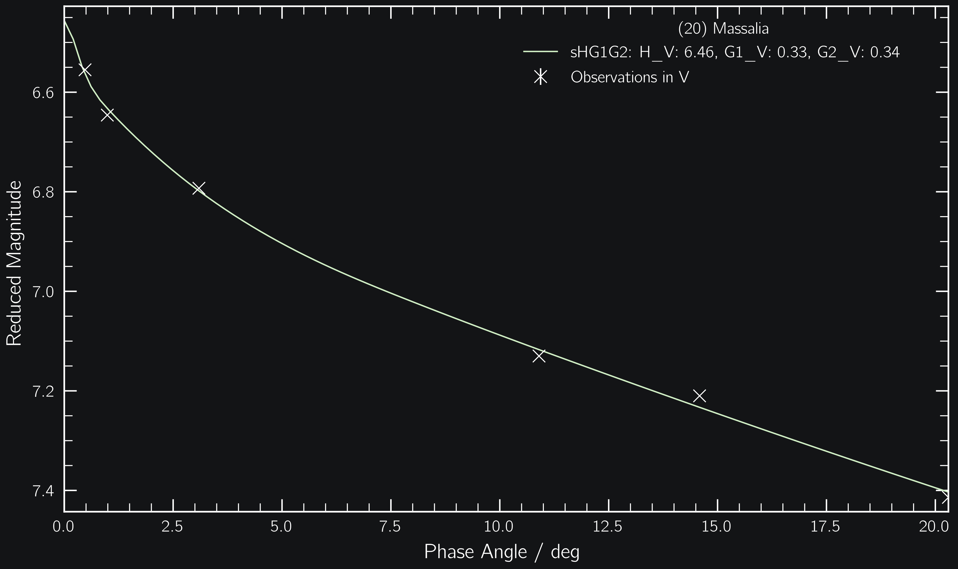
sHG1G2¶

From Carry+ 2024. phunk the model implementation from fink.

Note that the sHG1G2 model requires the target’s ephemerides at the time of observation. If you provide the target name and the epoch of observation, phunk queries the ephemerides for you from the IMCCE’s Miriade webservice.

import phunk

# Observations of (20) Massalia from Gehrels 1956
phase = [0.57, 1.09, 3.20, 10.99, 14.69, 20.42]
mag = [6.555, 6.646, 6.793, 7.130, 7.210, 7.414]

epoch = [35193, 35194, 35198, 35214, 35223, 35242]  # in MJD

pc = phunk.PhaseCurve(phase=phase, mag=mag, epoch=epoch, target=20)
pc.fit(['sHG1G2'])

pc.plot()

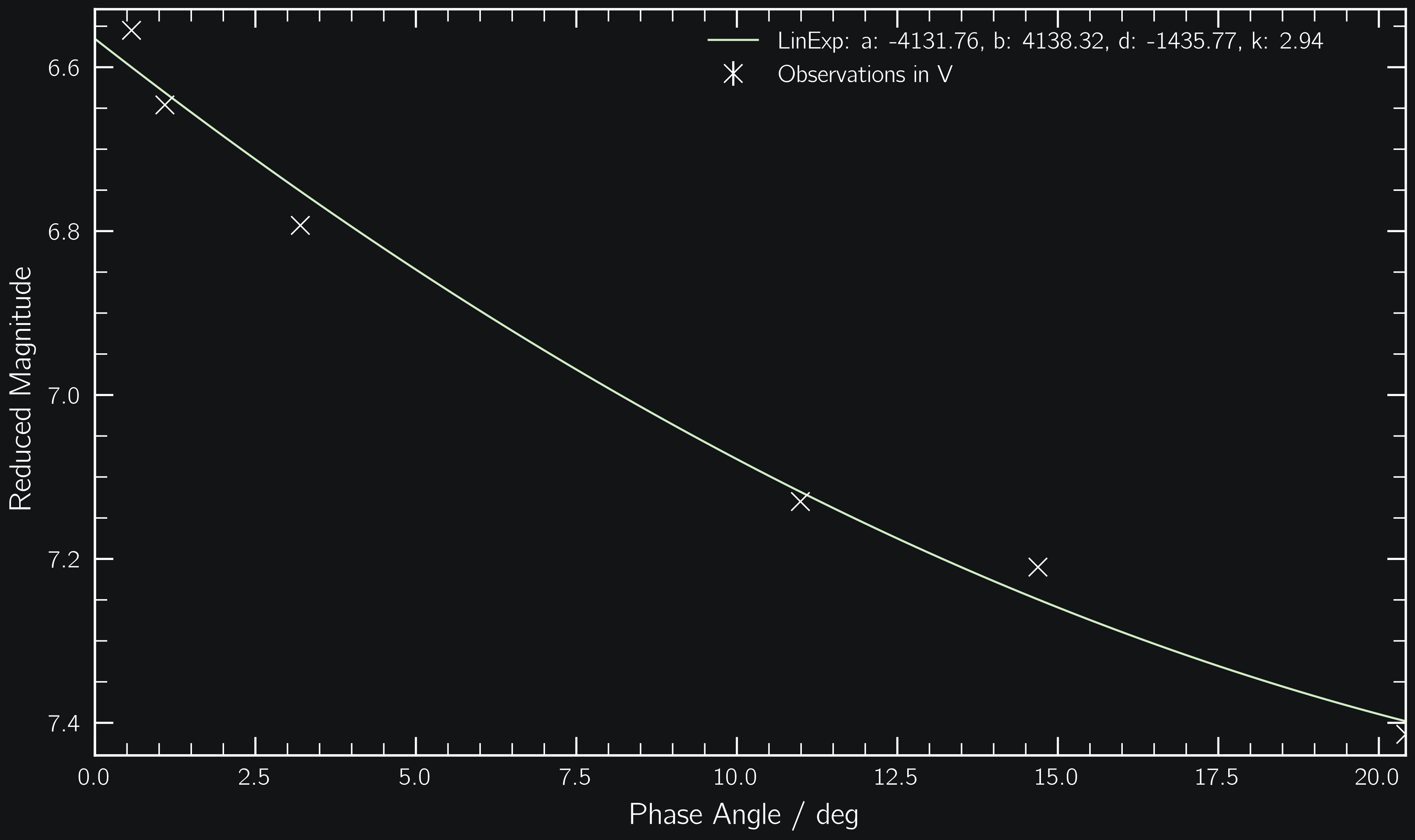
LinExp¶

Four-parameter linear-exponential model from Kaasalainen+ 2001.

\[f(\alpha) = a \exp(\frac{-\alpha}{d}) + k \alpha + b\]

with a and d the height and width of the opposition effect, k the photometric slope, and b the background.

import phunk

# Observations of (20) Massalia from Gehrels 1956
phase = [0.57, 1.09, 3.20, 10.99, 14.69, 20.42]
mag = [6.555, 6.646, 6.793, 7.130, 7.210, 7.414]

pc = phunk.PhaseCurve(phase=phase, mag=mag, target=20)
pc.fit(['LinExp'])

pc.plot()